3. Jupyter¶

3.1. What’s Jupyter?¶

The Jupyter project makes it possible to use code to experiment with and process data in your web browser. It lets you do all of these things in one page (or browser tab):

write and run code
write explanations of code and data, including with mathematical formulas
view tables, plots, and other visualizations of data
interact with certain types of data visualizations

It’s pronounced just like Jupiter, but has the funny spelling because it was originally built for Python, so they wanted to work a “py” in there somewhere.

You may prefer to use another tool to accomplish these tasks; your MA346 instructor won’t force you to use Jupyter. But you should still know about Jupyter for the following reasons:

Lots of people in data science and analytics use Jupyter notebooks, so you’ll definitely encounter them and want to be familiar with how to read them, edit them, and run them.
It’s becoming the lingua franca for how to share your data research online, so you may want to know how to publish Jupyter notebooks, something our course will cover.
It was a big enough deal to win one of the highest awards in the computer science profession, the 2017 ACM Software System Award.

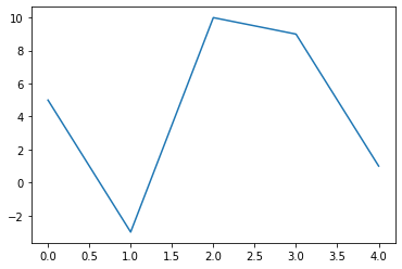
In fact, these course notes were written in Jupyter. That’s why you’ll see code inputs and outputs interspersed among them, because Jupyter lets you write documents with code built in, and it runs the code for you and shows you the output. Here’s an example:

import matplotlib.pyplot as plt
plt.plot( [5, -3, 10, 9, 1] )
plt.show()

Okay, sounds great, so where do we point our browser to start using this thing? Well, you’ve got lots of options, so let’s see what they are.

3.2. How does Jupyter work?¶

Before we dive into your options for using Jupyter, we need to understand Jupyter’s basic structure, so that we can appreciate the pros and cons of the available options.

Big Picture - The structure of Jupyter

Jupyter is made of two pieces:

The notebook interface, which shows you a document with code and visualizations in it, called “a Jupyter notebook.”
The engine behind the notebook, which runs your code, and is doing its work invisibly in the background; this engine is called the “kernel.”

How you interact with each of these two pieces is important, and comes with some pitfalls to avoid.

3.2.1. Jupyter in the cloud¶

The easiest way to start using Jupyter is to just point your browser at a website that offers you access to Jupyter in the cloud. In such a situation, Jupyter’s two pieces work like this:

The notebook interface runs in your browser on your computer
The kernel runs in the cloud on a server provided by someone else

Here are three examples of where you can use Jupyter notebooks in the cloud:

⭐ Best choice: Deepnote ⭐
- They took the standard Jupyter interface and added several new features.
- The amount of computing power they give you for free is pretty good (only once or twice in our course will we need more).
- It’s extremely easy to share your work with anyone.
- You and your instructor can even edit the same file at the same time and leave comments for one another, which is great when you need help on your work.
- While you’re a student, Deepnote is free to use.
- This is what your MA346 instructor will use almost all the time in class.
Next best choice: Google Colab
- Has many of the same positives as Deepnote except without the new interface features.
- Will not let you upload files; instead, you must take steps to connect it to your Google Drive.
Third choice: CoCalc
- Has many features that the previous two don’t have, including a nice palette of common code snippets you can insert.
- But the notebook interface is nonstandard and different from Jupyter’s in several ways.
- Is perhaps the most limited in terms of how much computing you get for free.

Obviously, none of these is going to give you access to a supercomputer for free. If you want to do any intense or lengthy computing in the cloud, you have to pay for them to let the kernel you’re using run on big hardware.

3.2.2. Jupyter on your machine¶

You can also choose to run Jupyter on your own machine. In contrast to accessing Jupyter in the cloud, when you run it on your own machine, Jupyter’s two pieces work like this:

The notebook interface still runs in your browser on your computer.
The kernel now also runs on your computer, which has both advantages and disadvantages.

As mentioned above, the huge benefits of using Jupyter in the cloud instead are that you don’t have to install anything on your computer or worry about the hassle of leaving a kernel running (which I explain below in the Big Picture box entitled “How to shut down Jupyter”). Furthermore, you can even access cloud providers on your phone or tablet, although that’s not typically desirable.

But there are just a few times in our course where you’ll want to have Python and all its data science tools installed on your local machine, because we’ll occasionally (though rarely) do an assignment that uses more computing power than cloud providers will give you for free. Typically you’ll want Jupyter installed as well, so I recommend installing it to be ready for those times. Also, if you have a poor wifi connection, you might want a local installation so that you don’t have to depend on the cloud for access to Jupyter.

There are several ways to install Jupyter on your computer, covered in each of the sections below.

3.2.3. Getting Jupyter through Anaconda¶

This is the easiest method for most people. See the page of these notes about installing Anaconda.

I recommend that you follow the optional instructions for installing VS Code as well, because you may prefer running Jupyter through VS Code. We’ll return to this topic below.
Once Anaconda is installed, you can launch it from the Windows Start menu or Mac Applications folder, then choose to launch either Jupyter Lab or the Jupyter Notebook.

Why are there two tools—Jupyter Lab and Jupyter notebook? Here’s the history:

Jupyter Notebook	Jupyter Lab
The original Jupyter project	Its newer successor
Uses multiple browser tabs	Does everything in one tab
Has no console/terminal access	Has both console and terminal access

Both technologies let you edit Jupyter notebooks. (Yes, it’s confusing that one app is called “the Jupyter Notebook” and the files are also called “Jupyter notebooks.” Sorry.) I recommend using Jupyter Lab.

Big Picture - How to shut down Jupyter

When you launch either the Jupyter Notebook or Jupyter Lab, you launch both the user interface (which you see in your browser) and the kernel (which you don’t see!). Just closing the browser tab does not close the kernel.

If you launch Jupyter repeatedly (e.g., each day in class) and never shut it down, you will have many copies of it running all at once on your computer, even if you cannot see them. This will slow your computer down. To prevent this, do one of these things every time you’re done using Jupyter:

From the Jupyter Notebook: File Menu > Close and Halt
From Jupyter Lab: File Menu > Shut down

These close the (invisible) kernel first, then let you close the user interface after that.

But that’s a hassle! Isn’t there an easier way? Yes, there are two easier ways, as the next two sections cover.

3.2.4. Getting Jupyter inside VS Code¶

In 2020, Microsoft significantly improved VS Code’s support for Jupyter notebooks so that VS Code (normally just a code editor) is a suitable environment in which to do all your data science work.

Jupyter notebook files are stored with the extension .ipynb, short for “IPython Notebook,” because the original name of the Jupyter project was IPython (I for interactive). You can double-click such a file to open it in VS Code, and edit it and run it right inside the VS Code app.

The biggest benefits of this method are these:

VS Code handles opening and closing a Jupyter kernel for you in the background. Just like when using a cloud provider, you don’t have to worry about shutting Jupyter down when you’re done using it.
Because Jupyter Notebook/Lab aren’t official apps you’ve installed on your machine, they can’t be launched when you double-click an .ipynb file. Instead, you have to manually open Jupyter Notebook/Lab first, then find the file. But VS Code is a real app, so it doesn’t have this drawback.
VS Code also has a built-in user interface for a tool called git, which we’ll learn a little bit about later in our course. If you’re using VS Code, you won’t have to install a separate app to work with git.

Great! So how do we get VS Code up and running? Here are two ways:

For most students: Use the Anaconda installation instructions mentioned above, and when you see the optional steps for installing VS Code, follow them. Anaconda gives you all the Python and data science tools you need, and VS Code will be the way you access them.
If you don’t want to change your existing Python setup: Some students may have Python installed, with a pre-existing set of packages, for another course or project, and don’t want to risk changing that setup. If so, you can use Docker instead of Anaconda to provide access to data science tools. Docker can be used to install a small virtual machine that’s pre-packaged with data science tools, kept separate from what’s already on your machine. See the instructions here if this is relevant to your needs.

Another editor that Anaconda ships with is Spyder. This project is very similar to VS Code, except that it is more tailored to the needs of data scientists, but is not as mature or widelyy-used a product in general. Students who are familiar with or prefer Spyder are welcome to use it as an alternative to VS Code.

3.2.5. Getting Jupyter through nteract¶

The final option is an app called nteract (pronounced like “interact”), which lets you access Jupyter notebooks in the same way you would access a Word or Excel document—by opening an app and seeing your notebook in a single window.

nteract requires you to have a working Python installation first. If you need one, install Anaconda before nteract, using the instructions referenced above.
Then visit the nteract website mentioned above and follow the very easy process of installing the nteract app.

nteract has many of the same benefits as VS Code’s Jupyter support, including handling the opening and closing of the kernel for you, and letting you double-click .ipynb files to open them in the nteract app. The nteract interface for notebooks is simpler and more straightforward than VS Code, but it does not have the built-in code-editing tools that VS Code has.

3.2.6. Which way should I choose?¶

That was a lot of information! Here’s a summary to help you decide how to proceed:

We’ll almost always use Deepnote in class, so unless you have a good reason not to, choose this cloud provider and get an account now.
You’ll occasionally want a Python-and-Jupyter installation on your own computer also, though we’ll use it less often than Deepnote. I recommend Anaconda with VS Code, so if you’re not sure which one to choose, choose that one. If you prefer one of the other options, that’s fine.

If you’re trying to decide whether to use a cloud provider or install Jupyter on your local machine, refer to the section above that discusses the pros and cons of each method. In this class, we will almost always use Deepnote during class, but for a few homework assignments you’ll want your own Jupyter installationn.

If you’re planning to use Jupyter in the cloud, see the section above that discusses the pros and cons of the various cloud platforms.

3.3. Closing comments¶

There are many websites that make it easy to view Jupyter notebooks online. This is very useful for sharing the results of your work when you’re done. Deepnote has powerful tools for this purpose, which we’ll explore in a future week. Other examples include NbViewer and GitHub, but there are many. Notebooks are often shared in nerdy places on the Internet, with websites supporting viewing them with all their plots, tables, and math displayed nicely. We will also learn how to use GitHub in a future week.

In your Python course (CS230), you probably used Python scripts (.py files) rather than Jupyter notebooks (.ipynb files). There are various pros and cons to these two formats. I will use notebooks throughout our course, because they are good for communicating, and communicating is my job. But if you want to write code in Python scripts, you can do so for most of the assignments in our course.

Learning on Your Own - Problems with Notebooks

Some folks really don’t like Jupyter notebooks. And they have good points! Study what pitfalls notebooks have, based on the presentation at that link, and report on them to the class.

Such a report would include:

From the many problems the presentation lists, choose the 4-6 that are most relevant to MA346 students.
For each such problem:
- Explain it carefully with a realistic example.
- Show how a tool other than Jupyter doesn’t have the same problem.
- Suggest specific ways that MA346 students can avoid pitfalls surrounding that problem.

Learning on Your Own - Math in Notebooks

You can add mathematics to Jupyter notebooks and it looks very nice. Here’s an example of the quadratic formula:

\[x=\frac{-b\pm\sqrt{b^2-4ac}}{2a}\]

This can be useful for explaining mathematical and statistical concepts in your work clearly, without resorting to ugly text attempts to look sort of like math. Study how you can add mathematical formulas to Markdown cells in Jupyter notebooks and report on it to the class.