6. Single-Table Verbs
See also the slides that summarize a portion of this content.
The functions we’ll discuss today got the name “verbs” because coders in the R community developed what they call a “grammar” for data transformation, and today’s content are some of that grammar’s “verbs.” The origins in R are unimportant for our course; what matters is that today’s topic is the actions you can do to a single table of data.
6.1. Tall and Wide Form
The following two tables show the same (fake) sales data, but in different forms. One is tall (6 rows, 4 columns) while the other is wide (2 rows, 5 columns).
Tall form:
First |
Last |
Day |
Sales |
|---|---|---|---|
Amy |
Smith |
Monday |
39 |
Amy |
Smith |
Tuesday |
68 |
Amy |
Smith |
Wednesday |
10 |
Bob |
Jones |
Monday |
93 |
Bob |
Jones |
Tuesday |
85 |
Bob |
Jones |
Wednesday |
0 |
Wide form:
First |
Last |
Monday |
Tuesday |
Wednesday |
|---|---|---|---|---|
Amy |
Smith |
39 |
68 |
10 |
Bob |
Jones |
93 |
85 |
0 |
Although it’s not a focus of this course, let me take a moment to mention a famous data-related concept. Data scientist and R developer Hadley Wickham wrote a paper called Tidy Data, which he defines as data with exactly one “observation” per row. (What an observation is depends on what you’ve gathered data about. In the first table above, an observation seems to be the amount of sales by a particular person on a particular day.) His rationale comes from people who’ve studied databases, and if you’ve taken CS350 at Bentley, you may be familiar with the related concept of database normal forms. The tidyverse is a collection of R packages that help you work smoothly with data if you organize it in tidy form.
Even though the details of tidy data aren’t part of our course, they’re closely related to whether data is stored in tall form or wide form (as shown in the two tables above).
Big Picture - The relationship between tall and wide data
Tall form is typically more useful when doing computations, because we often want to filter for just the rows we care about. So the more separated the data is into rows, the easier it is to select just the data we need.
Wide form is typically more useful when presenting data to humans. Although this tiny table is just an example, data in the real world has far more rows, meaning that the tall form will not fit on a page. Reshaping it into a rectangle that does fit on one page is easier to read.
We can convert between these forms.
Converting tall to wide is called pivoting.
Converting wide to tall is called melting.
Let’s investigate these two verbs.
6.2. Pivot
The box above says that pivot is the verb for converting tall-form data to wide-form data. We’ll give a precise definition later on. Let’s first get some intuition by looking at some pictures.
6.2.1. The general idea
The big picture idea of the pivot operation is illustrated here:
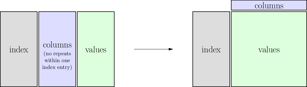
The table below shows the same fake sales data from earlier, in “tall” form. If you’re reading these notes online, you can drag the slider back and forth to see an animation of the transition from tall to wide form. While you do so, notice each of these parts:
The gray cells:
These are the unique IDs used in both forms, tall and wide.
They function like row headers.
In pandas, we call them the
indexof the pivot operation (which is not the same as the index of the DataFrame).
The blue cells:
These cells show the most important part of the pivot operation.
In tall form they’re entries in the table, but in wide form they’re column headers.
In pandas, we call them the
columnsof the pivot (because they become column headers when we pivot, even though they were table entries before).
The green cells:
Like the blue cells, these are also table entries, but are typically numbers.
Unlike the blue cells, they remain table entries, just moving to a new location or arrangement.
In pandas, we call them the
valuesof the pivot.
(The animation below can be viewed in its own page here.)
6.2.2. The precise definition
We can state precisely what df.pivot() does by building on what we’ve learned in previous chapters. We can describe both the requirements and guarantees of the pivot function, and can do so in terms of functions and relations.
Requirements of
df.pivot():The table to be pivoted must express a function from at least two input columns (called
indexandcolumns, above) to one output column (calledvalues, above).It is acceptable for the
indexto comprise more than one column, as in the example above.Recall that for it to be a function, inputs cannot be repeated, because that could connect them with more than one output.
Guarantees of
df.pivot():Each value from the
indexcolumns will appear only once in the resulting table (even if they were repeated in the input table).A new column will be created for each unique value in the old
columnscolumn.The
valuescolumn will have been removed.For each
indexentry \(i\) in the original DataFrame and eachcolumnsentry \(c\), if \(v\) is the unique value associated with it, then the new table will contain a row withindex\(i\) and with \(v\) in the column entitled \(c\). This is shown in the illustration below.
You can think of df.pivot() as turning one function into many. In the example above, it worked like this:
Inputs |
Output |
|||
|---|---|---|---|---|
Original table |
One function |
first name, last name, and day |
\(\to\) |
sales |
Result of pivoting |
First function |
first name and last name |
\(\to\) |
Monday sales |
Second function |
first name and last name |
\(\to\) |
Tuesday sales |
|
Third function |
first name and last name |
\(\to\) |
Wednesday sales |
6.2.3. Purpose of pivoting
Recall that pivoting just turns “tall” data into “wide” data. And tall form is how you typically store data when doing an analysis, because of the ease of processing tall data using code, while wide form is often more attractive for a human reading data from a table. So the purpose of pivoting is typically when you’re generating reports for human consumption.
6.3. Melt
The reverse operation to a pivot is called “melt.” This comes from the fact that wide data “falls down” (like the drips of a melting icicle, I guess?) into tall form. The idea is summarized in the following picture, but you can watch it happen in the animation further below.
6.3.1. The genreal idea
The big picture idea of the pivot operation is illustrated here:
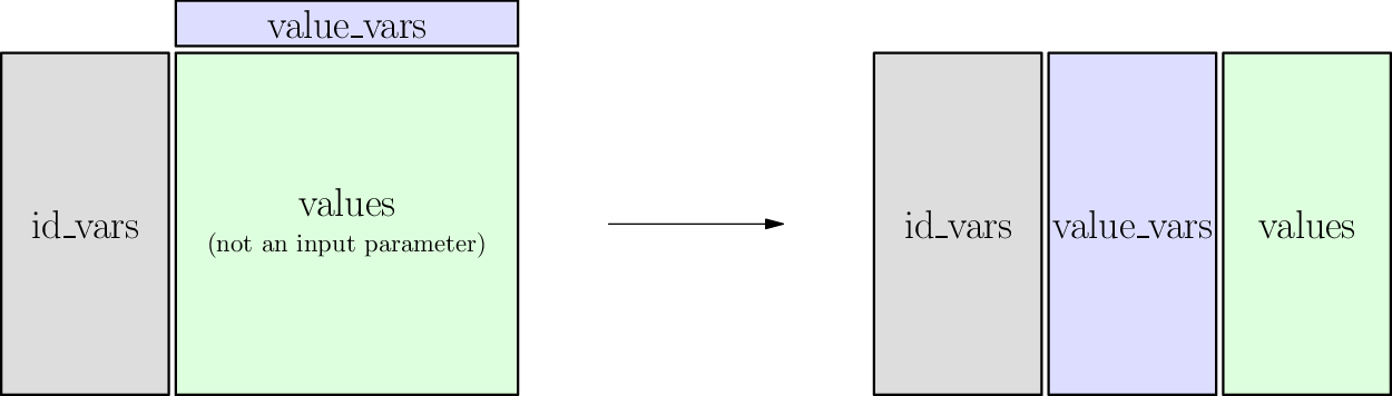
Just as pivoting was usually to turn data stored for computers into data readable by humans, melting is for the reverse. If you’re given data in wide form, but to prepare it for analysis, you often want to convert it into tall form to make subsequent data processing code easier.
For example, let’s say we were given the table below of students’ (fake) performance on various exams. We may prefer to have each exam as a separate observation, so that each row is a single exam score. To accomplish this, we can melt the table.
Drag the slider to see the melting in action. While you do so, watch the following parts of the table:
The gray cells:
Because we’ll be spreading a student’s data out over more than one row, these will be copied.
These function as unique IDs for each row, so pandas calls these columns the
id_vars.
The blue cells:
These are the row headings for each of several different functions.
Each function takes a student as input and gives a type of exam score as output.
They will change from being column headers to being values in the table, so pandas calls them the
value_vars.
The green cells:
Each column represents a separate function (the first maps students to SAT score, the second maps students to ACT score, and the third maps students to GPA).
Because we’re collecting all scores into a single column, these will stack up to become just one column.
(This animation can be viewed in its own page here.)
6.3.2. The precise definition
Unsurprisingly, the requirements and guarantees of the melt operation are the reverse of those from the pivot operation.
Requirements of
df.melt()The
id_varsare one or more columns that contain unique identifiers for each row.The
value_varscolumns are each a function from theid_vars. (That is, no value inid_varsappears twice.)
Guarantees of
df.melt()For each value \(i\) in the
id_varscolumn and for each column \(c\) in thevalue_vars, if \(v\) is the entry in that row and column, then the new table will contain a row with ID \(i\) and values \(c\) and \(v\).This new table will therefore be a function from the \(i\) and \(c\) columns to the \(v\) column. (By default, pandas calls those two new columns “variable” and “value” but you can give them more meaningful names.)
There are no rows in the resulting table besides those just described.
6.4. Pivot tables
All this talk of pivoting should remind you of the very common tool in Microsoft Excel (and many other applications, such as Tableau) called “pivot table.” It is very much like the pivot operation, with two differences. First, it doesn’t require the table to represent a function. Second, it does require you to explain how values will be summarized or combined. Naturally, pandas supports this operation as well, and it’s extremely useful.
If df.pivot() makes a tall table wide, then df.pivot_table() makes a tall table sort of wide. We’ll see why below.
6.4.1. The general idea
The big picture idea of the pivot operation is illustrated here:
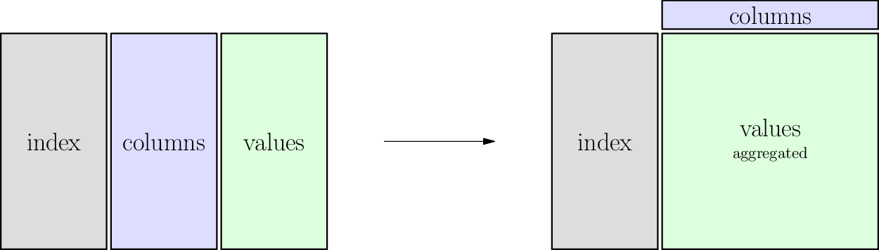
It’s worth looking back at the first section of this chapter and comparing this illustration to that one to note the two important differences.
In the table shown below, notice that if we try to consider the gray and blue columns as inputs and the green column as outputs, the relationship is not a function. If it were, we could pivot on the blue column, and the green cells would rearrange themselves just as they did in the first animation (in the Pivot section). But try dragging the slider below slowly and you will see that some green cells collide.
For instance, Amy Smith has two different sales to the same customer, Facebook, and Bob Jones has two different sales to the same customer, Amazon. So we cannot simply create a Facebook column and an Amazon column and rearrange the sales data into them. When two sales figures need to be placed under the same customer heading, we need some way to combine them.
The way the table below combines cells is by adding, which is a very sensible thing to do with sales data for a customer. You can see that the code asks this by specifying the aggregation function (or aggfunc) to be “sum.” But there are many aggregation functions, because “sum” is not always what you want; perhaps you wanted a report of average sales, or maximum sales, or something else. The DataCamp content you did in preparation for today covered other aggregation functions.
This is why a pivot_table operation doesn’t make a table that’s as wide as a pivot might, because some cells are combined, meaning that the overall table reduces in size.
(This animation can be viewed in its own page here.)
6.4.2. The precise definition
I will alter the precise definition of df.pivot() as little as possible when creating this definition of df.pivot_table().
Requirements of
df.pivot_table():The table to be pivoted can express any relation among least three columns (called
index,columns, andvalues, above).It is acceptable for the
indexto comprise more than one column, as in the example above. (Same as fordf.pivot().)We must have some aggregation function (called
aggfunc, above) that can combine many entries from thevaluescolumn into one. In the example above, we used “sum.” Let’s call this function \(A\).
Guarantees of
df.pivot_table():Each value from the
indexcolumns will appear only once in the resulting table. (Same as fordf.pivot().)A new column will be created for each unique value in the old
columnscolumn. (Same as fordf.pivot().)The
valuescolumn will have been removed. (Same as fordf.pivot().)For each
indexentry \(i\) in the original DataFrame and eachcolumnsentry \(c\), if \(v_1,v_2,\ldots,v_n\) are the various values associated with it, then the new table will contain a row withindex\(i\) and with \(A(v_1,v_2,\ldots,v_n)\) in the column entitled \(c\).
Since the pivot table operation is so familiar from Microsoft Excel, now would be a good time to mention two Excel-related Learning on Your Own projects:
Learning on Your Own - Mito
A new startup company called Mito lets you use an online spreadsheet to generate Python code for manipulating dataframes. Investigate the product and give a report that answers all of the following questions.
Could students in our class benefit from using Mito?
What are the most interesting/useful/powerful actions that Mito supports and for which it can construct Python code? (For example, can it do all of the contents of this chapter, or not?)
If a student in our class wanted to get started using Mito, how should they do so? (I.e., what do they need to install, and how do they get the results back into their own notebooks or Python projects?)
What are the current limitations of Mito?
Learning on Your Own - xlwings
xlwings is a product for connecting Python with Excel. Investigate the product and give a report that answers all of the following questions.
For students of Python, what new powers does xlwings give you for accessing Excel?
Give an example (including code, an Excel workbook, and specific instructions) of how one of your classmates could use Python to control Excel.
For users of Excel, what new powers does xlwings give you for leveraging Python?
Give an example (including code, an Excel workbook, and specific instructions) of how one of your classmates could use Excel to leverage Python.
Which of xlwings’s features do you think are most applicable or attractive for MA346 students?
6.5. Stack and unstack
There are two other single-table verbs that you studied in the DataCamp review before today’s reading. These are less common because they apply only in the context where there is a multi-index, either on rows or columns. But we give animations of each below to help the reader visualize them.
The stack operation takes nested column indices (which are arranged horizontally) and makes them nested row indices (which are arranged vertically). This is why it’s called “stack,” because it arranges the headings vertically. Unstack is the same operation in reverse.
When applying these operations, it is possible to choose which level of a multi-index gets stacked or unstacked. The two animations below use two different levels, so that you can compare the differences.
6.5.1. Animation for unstack/stack at level 1
The level of a stack/unstack operation refers to which level of the multi-index will be moved. The animation below shows df.unstack( level=1 ) when you move the slider from left to right, so level 1 of the row multi-index (the weeks) moves up to become part of the column index. It is always placed as an inner index, but this can be changed afterwards with df.swaplevel().
The reverse operation is exactly df.stack( level=1 ), because it moves level 1 from the column headings back to be inside the row headings instead.
(This animation can be viewed in its own page here.)
6.5.2. Animation for unstack/stack at level 0
The level of a stack/unstack operation refers to which level of the multi-index will be moved. The animation below shows df.unstack( level=0 ) when you move the slider from left to right, so level 0 of the row multi-index (the months) moves up to become part of the column index. It is always placed as an inner index, but this can be changed afterwards with df.swaplevel().
The reverse operation is therefore actually a combination of df.stack() (which would put the months inside the weeks) and df.swaplevel() (which would fix that) all in one.
(This animation can be viewed in its own page here.)