9. Mathematics and Statistics in Python
See also the slides that summarize a portion of this content.
9.1. Math in Python
Having had CS230, you are surely familiar with Python’s built-in math operators +, -, *, /, and **. You’re probably also familiar with the fact that Python has a math module that you can use for things like trigonometry.
import math
math.cos( 0 )
1.0
I list here just a few highlights from that module that are relevant for statistical computations.
math.exp(x) is \(e^x\), so the following computes \(e\).
math.exp( 1 )
2.718281828459045
Natural logarithms are written \(\ln x\) in mathematics, but just log in Python.
math.log( 10 ) # natural log of 10
2.302585092994046
A few other functions in the math module are also useful for data work, but show up much less often. The distance between any two points in the plane (or any number of dimensions) can be computed with math.dist().
math.dist( (1,0), (-5,2) )
6.324555320336759
Combinations and permutations can be computed with math.comb() and math.perm() (since Python 3.8).
9.2. Naming mathematical variables
In programming, we almost never name variables with unhelpful names like k and x, because later readers of the code (or even ourselves reading it in two months) won’t know what k and x actually mean. The one exception to this is in mathematics, where it is normal to use single-letter variables, and indeed sometimes the letters matter.
Example 1: The quadratic formula is almost always written using the letters \(a\), \(b\), and \(c\). Yes, names like x_squared_coefficient, x_coefficient, and constant are more descriptive, but they would lead to much uglier code that’s not what anyone expects. Compare:
# not super easy to read, but not bad:
def quadratic_formula_1 ( a, b, c ):
    solution1 = ( -b + ( b**2 - 4*a*c )**0.5 ) / ( 2*a )
    solution2 = ( -b - ( b**2 - 4*a*c )**0.5 ) / ( 2*a )
    return ( solution1, solution2 )

# oh my make it stop:
def quadratic_formula_2 ( x_squared_coefficient, x_coefficient, constant ):
    solution1 = ( -x_coefficient + \
                    ( x_coefficient**2 - 4*x_squared_coefficient*constant )**0.5 ) \
                  / ( 2*x_squared_coefficient )
    solution2 = ( -x_coefficient - \
                    ( x_coefficient**2 - 4*x_squared_coefficient*constant )**0.5 ) \
                  / ( 2*x_squared_coefficient )
    return ( solution1, solution2 )

# of course both work fine:
quadratic_formula_1(3,-9,6), quadratic_formula_2(3,-9,6)
((2.0, 1.0), (2.0, 1.0))
But the first one is so much easier to read.
Example 2: Statistics always uses \(\mu\) for the mean of a population and \(\sigma\) for its standard deviation. If we wrote code where we used mean and standard_deviation for those, that wouldn’t be hard to read, but it wouldn’t be as clear, either.
Interestingly, you can actually type Greek letters into Python code and use them as variable names! In Jupyter, just type a backslash (\) followed by the name of the letter (such as mu) and then press the Tab key. It will replace the code \mu with the actual letter \(\mu\). I’ve done so in the example code below.
def normal_pdf ( μ, σ, x ):
    """The value of the probability density function for
    the normal distribution N(μ,σ^2), with mean μ and
    variance σ^2."""
    shifted = ( x - μ ) / σ
    return math.exp( -shifted**2 / 2.0 ) \
         / math.sqrt( 2*math.pi ) / σ

normal_pdf( 10, 2, 15 )
0.00876415024678427
The same feature is not (yet?) available in VS Code, but you can copy and paste Greek letters from anywhere into your code in any editor, and they still count as valid Python variable names.
9.3. But what about NumPy?
Pandas is built on NumPy, and many data science projects also use NumPy directly. Since NumPy implements tons of mathematical tools, why bother using the ones in Python’s built-in math module? Well, on the one hand, NumPy doesn’t have everything; for instance, the math.comb() and math.perm() functions mentioned above don’t exist in NumPy. But when you can use NumPy, you should, for the following important reason.
Big Picture - Vectorization and its benefits
All the functions in NumPy are vectorized, meaning that they will automatically apply themselves to every element of a NumPy array. For instance, you can just as easily compute square(5) (and get 25) as you can compute square(x) if x is a list of 1000 entries. NumPy notices that you provided a list of things to square, and it squares them all. What are the benefits to vectorization?
Using vectorization saves you the work of writing loops. You don’t have to loop through all 1000 entries in
xto square each one; NumPy knew what you meant.Using vectorization saves the readers of your code the work of reading and understanding loops.
If you had to write a loop to apply a Python function (like
lambda x: x**2) to a list of 1000 entries, then the loop would (obviously) run in Python. Although Python is a very convenient language to code in, it does not produce very fast-running code. Tools like NumPy are written in languages like C++, which are less convenient to code in, but produce faster-running results. So if you can have NumPy automatically loop over your data, rather than writing a loop in Python, the code will execute faster.
We will return to vectorization and loops in Chapter 11 of these notes. For now, let’s just run a few NumPy functions. In each case, notice that we give it an array as input, and it automatically knows that it should take action on each entry in the array.
# Create an array of 30 random numbers to work with.
import numpy as np
values = np.random.rand( 30 )
values
array([0.1328306 , 0.34671288, 0.67541447, 0.00693541, 0.26074135,
       0.87412487, 0.7968968 , 0.50565012, 0.91904316, 0.14921354,
       0.73448094, 0.10871186, 0.44963219, 0.33382355, 0.60418287,
       0.87072846, 0.11232413, 0.30544017, 0.91011315, 0.17641629,
       0.97928091, 0.03727242, 0.09603148, 0.78404571, 0.67176734,
       0.0762971 , 0.19615451, 0.11717903, 0.4470815 , 0.18233837])
np.around( values, 2 ) # round to 2 decimal digits
array([0.13, 0.35, 0.68, 0.01, 0.26, 0.87, 0.8 , 0.51, 0.92, 0.15, 0.73,
       0.11, 0.45, 0.33, 0.6 , 0.87, 0.11, 0.31, 0.91, 0.18, 0.98, 0.04,
       0.1 , 0.78, 0.67, 0.08, 0.2 , 0.12, 0.45, 0.18])
np.exp( values ) # compute e^x for each x in the array
array([1.14205652, 1.41441056, 1.96484718, 1.00695952, 1.29789192,
       2.39677689, 2.21864533, 1.65806311, 2.50689055, 1.16092087,
       2.08439979, 1.11484108, 1.56773545, 1.39629675, 1.82975645,
       2.38865026, 1.11887547, 1.35722228, 2.48460366, 1.19293456,
       2.66254095, 1.03797574, 1.10079372, 2.19031576, 1.95769417,
       1.07928318, 1.21671488, 1.12432069, 1.56374175, 1.20002018])
np.square( values ) # square each value
array([1.76439689e-02, 1.20209822e-01, 4.56184706e-01, 4.80999385e-05,
       6.79860509e-02, 7.64094294e-01, 6.35044508e-01, 2.55682041e-01,
       8.44640329e-01, 2.22646813e-02, 5.39462257e-01, 1.18182690e-02,
       2.02169103e-01, 1.11438166e-01, 3.65036940e-01, 7.58168054e-01,
       1.26167109e-02, 9.32936952e-02, 8.28305954e-01, 3.11227075e-02,
       9.58991102e-01, 1.38923297e-03, 9.22204583e-03, 6.14727683e-01,
       4.51271357e-01, 5.82124768e-03, 3.84765904e-02, 1.37309242e-02,
       1.99881872e-01, 3.32472817e-02])
Notice that this makes it very easy to compute certain mathematical formulas. For example, when we want to measure the quality of a model, we might compute the RSSE, or Root Sum of Squared Errors, that is, the square root of the sum of the squared differences between each actual data value \(y_i\) and its predicted value \(\hat y_i\). In math, we write it like this:
The summation symbol lets you know that a loop will take place. But in NumPy, we can do it without writing any loops.
ys    = np.array( [ 1, 2, 3, 4, 5 ] )   # made up data
yhats = np.array( [ 2, 1, 0, 3, 4 ] )   # also made up
RSSE  = np.sqrt( np.sum( np.square( ys - yhats ) ) )
RSSE
3.605551275463989
Notice how the NumPy code also reads just like the English: It’s the square root of the sume of the squared differences; the code literally says that in the formula itself! If we had had to write it in pure Python, we would have used either a loop or a list comprehension, like in the example below.
RSSE = math.sqrt( sum( [ ( ys[i] - yhats[i] )**2 for i in range(len(ys)) ] ) ) # not as readable
RSSE
3.605551275463989
A comprehensive list of NumPy’s math routines appear in the NumPy documentation.
9.4. Binding function arguments
Many functions in statistics have two types of parameters. Some of the parameters you change very rarely, and others you change all the time.
Example 1: Consider the normal_pdf function whose code appears in an earlier section of this chapter. It has three parameters, \(\mu\), \(\sigma\), and \(x\). You’ll probably have a particular normal distribution you want to work with, so you’ll choose \(\mu\) and \(\sigma\), and then you’ll want to use the function on many different values of \(x\). So the first two parameters we choose just once, and the third parameter changes all the time.
Example 2: Consider fitting a linear model \(\beta_0+\beta_1x\) to some data \(x_1,x_2,\ldots,x_n\). That linear model is technically a function of three variables; we might write it as \(f(\beta_0,\beta_1,x)\). But when we fit the model to the data, then \(\beta_0\) and \(\beta_1\) get chosen, and we don’t change them after that. But we might plug in hundreds or even thousands of different \(x\) values to \(f\), using the same \(\beta_0\) and \(\beta_1\) values each time.
Programmers have a word for this; they call it binding the arguments of a function. Binding allows us to tell Python that we’ve chosen values for some parameters and won’t be changing them; Python can thus give us a function with fewer parameters, to make things simpler. Python does this with a tool called partial in its functools module. Here’s how we would apply it to the normal_pdf function.
from functools import partial

# Let's say I want the standard normal distribution, that is,
# I want to fill in the values μ=0 and σ=1 once for all.
my_pdf = partial( normal_pdf, 0, 1 )

# now I can use that on as many x inputs as I like, such as:
my_pdf( 0 ), my_pdf( 1 ), my_pdf( 2 ), my_pdf( 3 ), my_pdf( 4 )
(0.3989422804014327,
 0.24197072451914337,
 0.05399096651318806,
 0.0044318484119380075,
 0.00013383022576488537)
In fact, SciPy’s built-in random number generating procedures let you use them either by binding arguments or not, at your preference. For instance, to generate 10 random floating point values between 0 and 100, we can do the following. (The rvs function stands for “random values.”)
import scipy.stats as stats
stats.uniform.rvs( 0, 100, size=10 )
array([22.02653725, 41.59178897, 17.51279454,  3.90432364, 67.0462826 ,
       49.60387328, 51.75750444, 45.80307533, 23.19363314, 31.08095795])
Or we can use built-in SciPy functionality to bind the first two arguments and create a specific random variable, then call rvs on that.
X = stats.uniform( 0, 100 )  # make a random variable
X.rvs( size=10 )             # generate 10 values from it
array([46.15255999, 51.52065162, 46.1135549 , 87.89082754, 14.29183601,
       84.47318685, 20.38114   , 10.89102008, 13.47299113, 62.1850617 ])
The same random variable can, of course, be used to create more values later.
The partial tool built into Python only works if you want to bind the first arguments of the function. If you need to bind later ones, then you can do it yourself using a lambda, as in the following example.
def subtract ( a, b ):   # silly little example function
    return a - b

subtract_1 = lambda a: subtract( a, 1 )  # bind second argument to 1

subtract_1( 5 )
4
We will also use the concept of binding function parameters when we come to curve fitting at the end of this chapter.
9.5. GB213 in Python
All MA346 students have taken GB213 as a prerequisite, and we will not spend time in our course reviewing its content. However, you may very well want to know how to do computations from GB213 using Python, and these notes provide an appendix that covers exactly that. Refer to it whenever you need to use some GB213 content in this course.
Topics covered there:
Discrete and continuous random variables
creating
plotting
generating random values
computing probabilities
computing statistics
Hypothesis testing for a population mean
one-sided
two-sided
Simple linear regression (one predictor variable)
creating the model from data
computing \(R\) and \(R^2\)
visualizing the model
That appendix does not cover the following topics.
Basic probability (covered in every GB213 section)
ANOVA (covered in some GB213 sections)
\(\chi^2\) tests (covered in some GB213 sections)
Learning on Your Own - Pingouin
The GB213 review appendix that I linked to above uses the very popular Python statistics tools statsmodels and scipy.stats. But there is a relatively new toolkit called Pingouin; it’s not as popular (yet?) but it has some advantages over the other two. See this blog post for an introduction and consider a tutorial, video, presentation, or notebook for the class that answers the following questions.
For what tasks is Pingouin better than
statsmodelsorscipy.stats? Show example code for doing those tasks in Pingouin.For what tasks is Pingouin less useful or not yet capable, compared to the others?
If I want to use Pingouin, how do I get started?
9.6. Curve fitting in general
The final topic covered in the GB213 review mentioned above is simple linear regression, which fits a line to a set of (two-dimensional) data points. But Python’s scientific tools permit you to handle much more complex models. We cannot cover mathematical modeling in detail in MA346, because it can take several courses on its own, but you can learn more about regression modeling in particular in MA252 at Bentley. But we will cover how to fit an arbitrary curve to data in Python.
9.6.1. Let’s say we have some data…
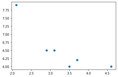
We will assume you have data stored in a pandas DataFrame, and we will lift out just two columns of the DataFrame, one that will be used as our \(x\) values (independent variable), and the other as our \(y\) values (dependent variable). I’ll make up some data here just for use in this example.
# example data only, totally made up:
import pandas as pd
df = pd.DataFrame( {
    'salt used (x)' :     [ 2.1, 2.9, 3.1, 3.5, 3.7, 4.6 ],
    'ice remaining (y)' : [ 7.9, 6.5, 6.5, 6.0, 6.2, 6.0 ]
} )
df
| salt used (x) | ice remaining (y) | |
|---|---|---|
| 0 | 2.1 | 7.9 |
| 1 | 2.9 | 6.5 |
| 2 | 3.1 | 6.5 |
| 3 | 3.5 | 6.0 |
| 4 | 3.7 | 6.2 |
| 5 | 4.6 | 6.0 |
import matplotlib.pyplot as plt
xs = df['salt used (x)']
ys = df['ice remaining (y)']
plt.scatter( xs, ys )
plt.show()
9.6.2. Choose a model
Curve-fitting is a powerful tool, and it’s easy to misuse it by fitting to your data a model that doesn’t make sense for that data. A mathematical modeling course can help you learn how to assess the appropriateness of a given type of line, curve, or more complex model for a given situation. But for this small example, let’s pretend that we know that the following model makes sense, perhaps because some earlier work with salt and ice had success with it. (Again, keep in mind that this example is really, truly, totally made up.)
We will use this model. When you do actual curve-fitting, do not use this model. It is a formula I crafted just for use in this one specific example with made-up data. When fitting a model to data, choose an appropriate model for your data.
Obviously, it’s not the equation of a line, so linear regression tools like those covered in the GB213 review notebook won’t be sufficient. To begin, we code the model as a Python function taking inputs in this order: first, \(x\), then after it, all the model parameters \(\beta_0,\beta_1\), and so on, however many model parameters there happen to be (in this case three).
def my_model ( x, β0, β1, β2 ):
    return β0 / ( β1 + x ) + β2
9.6.3. Ask SciPy to find the \(\beta\)s
This step is called “fitting the model to your data.” It finds the values of \(\beta_0,\beta_1,\beta_2\) that make the most sense for the particular \(x\) and \(y\) data values that you have. Using the language from earlier in this chapter, SciPy will tell us how to bind values to the parameters \(\beta_0,\beta_1,\beta_2\) of my_model so that the resulting function, which just takes x as input, is the one best fit to our data.
For example, if we picked our own values for the model parameters, we would probably guess poorly. Let’s try guessing \(\beta_0=3,\beta_1=4,\beta_2=5\).
# fill in my guesses for the β parameters:
guess_model = lambda x: my_model( x, 3, 4, 5 )

# plot the data:
plt.scatter( xs, ys )

# plot my model by sampling many x values on it:
many_xs = np.linspace( 2, 5, 100 )
plt.plot( many_xs, guess_model( many_xs ) )

# show the two plots together:
plt.show()
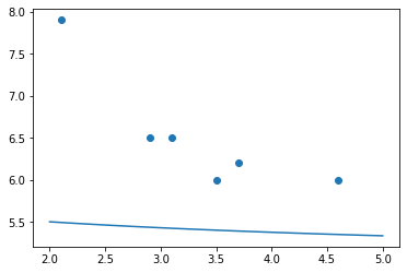
Yyyyyyeah… Our model is nowhere near the data. That’s why we need SciPy to find the \(\beta\)s. Here’s how we ask it to do so. You start with your own guess for the parameters, and SciPy will improve it.
from scipy.optimize import curve_fit
my_guessed_betas = [ 3, 4, 5 ]
found_betas, covariance = curve_fit( my_model, xs, ys, p0=my_guessed_betas )
β0, β1, β2 = found_betas
β0, β1, β2
(1.3739384272240622, -1.5255461192343747, 5.510233385761209)
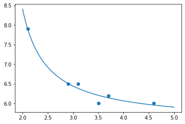
So how does SciPy’s found model look?
9.6.4. Describe and show the fit model
Rounding to a few decimal places, our model is therefore the following:
It fits the data very well, as you can see below.
fit_model = lambda x: my_model( x, β0, β1, β2 )
plt.scatter( xs, ys )
plt.plot( many_xs, fit_model( many_xs ) )
plt.show()
Big Picture - Models vs. fit models
In mathematical modeling and machine learning, we sometimes distinguish between a model and a fit model.
Models are general descriptions of how a real-world system behaves, typically expressed using mathematical formulas. Each model can be used on many datasets, and a statistician or data scientist does the work of choosing the model they think suits their data (and often also choosing which variables from the data are relevant).
Example models:
A linear model, \(y=\beta_0+\beta_1x\)
A quadratic model, \(y=\beta_0+\beta_1x+\beta_2x^2\)
A logistic curve, \(y=\frac{\beta_0}{1+e^{\beta_1(-x+\beta_2)}}\)
A neural network
A fit model is the specific version of the general model that’s been tailored to suit your data. We create it from the general model by binding the values of the \(\beta\)s to specific numbers.
For example, if your model were \(y=\beta_0+\beta_1x\), then your fit model might be \(y=-0.95+1.13x\). In the general model, \(y\) depends on three variables (\(x,\beta_0,\beta_1\)). In the fit model, it depends on only one variable (\(x\)). So model fitting is an example of binding the variables of a function.
When speaking informally, a data scientist or statistician might not always distinguish between “model” and “fit model,” sometimes just using the word “model” and expecting the listener to know which one is being discussed. In other words, you will often hear people not bother with fussing over the specific technical terminology I just introduced.
But when we’re coding or writing mathematical formulas, the difference between a model and a fit model will always be clear. The model in the example above was a mathematical formula with \(\beta\)s in it, and a Python function called my_model, that had β parameters. But the fit model was the result of asking SciPy to do a curve_fit, and in that result, all the \(\beta\)s had been replaced with actual values. That’s why we named that result fit_model.
The final chapter in these course notes does a preview of machine learning, using the popular Python package scikit-learn. Here’s a little preview of what it looks like to fit a model to data using scikit-learn. It’s not important to fully understand this code right now, but just to notice that scikit-learn makes the distinction between models and fit models impossible to ignore.
# Let's say we're planning to use a linear model.
from scklearn.linear_model import LinearRegression
model = LinearRegression()
# We now have a model, but not a fit model.
# We can't ask what its coefficients are, because they don't exist yet.

# I want to find the best linear model for *my* data.
model.fit( df['my independent variable'], df['my dependent variable'] )
# We now have a fit model.
# If we asked for its coefficients, we would see actual numbers.
In class, we will use the SciPy model-fitting technique above to fit a logistic growth model to COVID-19 data. Be sure to have completed the preparatory work on writing a function that extracts the series of COVID-19 cases over time for a given state! Recall that it appears on the final slide of the Chapter 8 slides.